Biologists possess the detailed knowledge critical for extracting biological insight from genome-wide data resources and yet they are increasingly faced with non-trivial computational analysis challenges posed by genome-scale methodologies. To lower this computational barrier, particularly in the early data exploration phases, we have developed an interactive pattern discovery and visualization approach, Spark, designed with epigenomic data in mind.
If you like Spark you may want to try our related tool ChAsE (Chromatin Analysis and Exploration). It incorporates the same principle of clustering across regions of interest, but introduces an interactive sortable heat map view and the ability to construct region sets based on presence/absence of signal. You can read more about it in the companion paper.
Visit the ChAsE website » Read the paper »
Spark is also available as a service within the Epigenome toolset of the Genboree Workbench. This Genboree deployment enables analysis of any private or public data hosted at Genboree. It also supports simultaneous processing of multiple Spark clustering analyses, which is not currently supported by the standalone tool.
Go to Genboree » Watch the video »
Genome browsers are ideal for viewing local regions of interest.
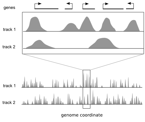
Many genomics techniques produce measurements that have both a value and a position on a reference genome, for example ChIP-sequencing. Popular genome browsers arrange the linear genome coordinate along the x axis and express the data value range on the y axis. This approach enables integration of diverse data sets by plotting them as vertically stacked tracks across a common genomic x axis. Genome browsers are designed for viewing local regions of interest (e.g. an individual gene) and are frequently used during the initial data inspection and exploration phases.
But they do not provide a global overview of these regions.
Most genome browsers support zooming along the genome coordinate. This type of overview is not always useful because it produces a summary across a continuous genomic range (e.g. chromosome 1) and not across the subset of regions that are of interest (e.g. genes on chromosome 1). There is a need for tools that help answer questions like: "What are the common data patterns across genes start sites in my data set?"
Achieve meaningful overview and detail by focusing on regions of interest
Step 1: Pre-processing
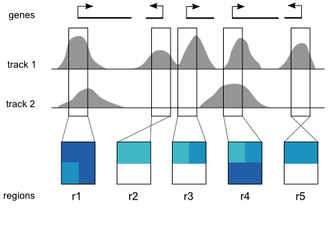
A Spark analysis begins with two user inputs: (i) one or more data tracks, and (ii) a set of regions of interest. Spark extracts a data matrix for each input region and orients it according to strand. Rows in these matrices correspond to data tracks and columns represent data bins along the genomic x-axis (two bins per region are used the diagram). The values are then normalized between 0 and 1 that can be visualized as heatmaps.

Step 2: Clustering
The preprocessed data are then clustered using k-means clustering using a user specified number of clusters (k). This technique was chosen for its effectiveness, relative simplicity, and runtime speed.
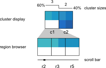
Step 3: Interactive visualization
The visualization is composed of two components: the Cluster Display, which provides a summary of each cluster, and the Region Browser, which displays individual cluster members. The user can therefore see both a high-level picture of the patterns in their data, while also being able to drill-down to individual regions of interest. The low-level region view is supported by links out to the UCSC Genome Browser, and the high-level cluster view supports interactive analyses such as manual cluster refinement and links out to the DAVID gene ontology tool set.
This video illustrates Spark's core features, including (1) how to cluster your data and data available from the Human Epigenome Atlas, (2) how to interactively refine clusters, and (3) how to connect to the UCSC Genome Browser and DAVID gene ontology tools.
This video can be downloaded here.
Spark is a clustering and visualization tool that enables the interactive exploration of genome-wide data. It is intended to "spark" insights into genome-scale data sets. The approach utilizes data clusters as a high-level visual guide and supports interactive inspection of individual regions within each cluster. The cluster view links to gene ontology analysis tools and the detailed region view connects to existing genome browser displays taking advantage of their wealth of annotation and functionality.
There are two ways to get a feeling for Spark without generating your own clustering:
1. Download Spark and follow the Example icon on Spark's opening screen to load an example clustering.

2. Watch the Spark video tutorial available under the Videos tab. This same video is available by following the Video icon on Spark's opening screen. It uses the same data set as in the example clustering mentioned above.
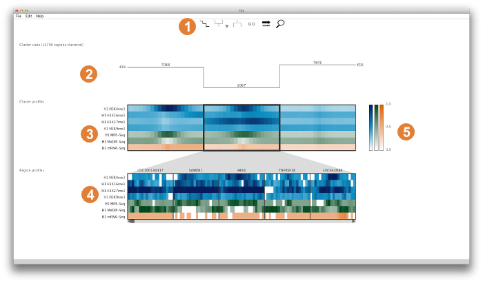
Core elements

This panel provides access to cluster summary options, cluster split and merge operations, external GO analysis tools, region sorting options, and a search box that dynamically searches for a region by name. More details on these individual controls are given below in the Detailed Look at the Control Panel.

This panel gives an overview of the cluster properties. The overview has three alternative forms: (1) graphs of cluster size, (2) split/merge path, or (3) histograms of the distances between regions in a cluster and the cluster's centroid. These graphs serve as useful guides to browsing and manipulating the clusters. More information on each graph type can be found below in the Detailed Look at the Control Panel.

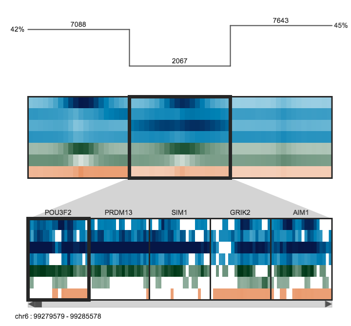
The upper panel displays the clusters as heatmaps (three clusters are shown in the above example). Each cluster heatmap displays the average values of its member regions and thus provides a global overview of its member patterns. Rows correspond to data samples ("tracks") and columns represent genomic bins. The number of bins can be specified by the user (e.g. 20 bins are used in the above example). Sample names are displayed to the left; if there are too many to display, then these names are available on mouseover only. Clusters are initially arranged in descending order by number of member regions.

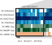
The Region Browser is a scrollable panel in which the individual members of the currently selected cluster can be explored. Only five regions are displayed at one time. If the "Name" attribute was specified in the regions file, then these names will appear above the corresponding regions and are also searchable in the search box. If the names are too long to be displayed without overlaps, then they are made be available upon mouseover, as is done for the sample names. The region coordinate is always available on mouseover only.

Normalized data values (range: 0.0 - 1.0) are mapped onto a colour gradient for display. The same colour gradient is used for heatmaps in the Cluster Display and Region Browser.
A Detailed Look at the Control Panel
Cluster Summary
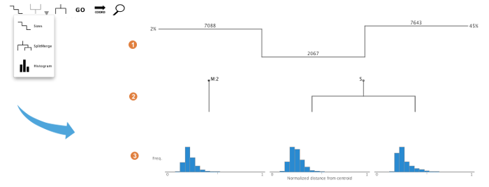
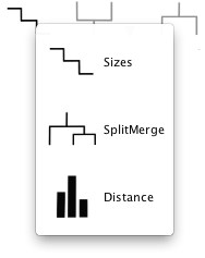
A size bar is drawn above the clusters and displays the absolute number of region members in each cluster. The total number of regions is reported on the far left in the title.
A tree outlines the path of cluster split and merge operations that have happened over the course of the analysis. Branch points are indicated with S and M. S on a node indicates a split. M on a node indicates a merge. The tree also keeps track of the number of merges on a particular node indicated by M:(number of merged clusters). A total number of split and merge operations are kept track in the title field above the tree.
Histograms are displayed showing the frequency of regions in each cluster, from 0% to 100%, of the global maximum Euclidean distance calculated between regions and their corresponding cluster centroids. This histogram is valuable in interpreting the tightness of the distribution within a cluster in comparison to other clusters. The distribution can be a helpful guide towards decisions on splitting and merging clusters. When using the region browser with the histogram, the region's position within the cluster is indicated by a triangular marker.
Cluster and Feature Operations

To split a cluster within the visualization tool, click on the target cluster and select the "split cluster" control panel option (image on the left). This will launch a new k=2 k-means clustering using only the regions within the selected cluster, effectively splitting it into two new clusters. While the clustering is running, the target cluster will appear grey. However, the clustering is performed on a separate thread, so you can still interact with the unaffected clusters.

To merge clusters within the visualization tool, first select multiple clusters. This can be achieved in two ways:
1) ctrl + click, which selects only the clusters being clicked, or
2) shift + (click + click), which selects all the clusters within the range of the 2 clicks.
Clicking on the merge button will by default merge the results into the left-most cluster. However, if you wish to specify a destination cluster, then click on the arrow beside the merge button to
bring up a list of possible destination clusters.
Like cluster split, while the clustering is running, the target cluster will appear grey. However, the clustering is performed on a separate thread, so you can still interact with the unaffected clusters.

Click on the GO control panel option to launch a GO analysis using the regions within the currently selected cluster. This will upload the region ids from the selected cluster to the DAVID website, enabling you to view GO classifications. This option only functions if the input GFF3 regions file contains the attribute "ID".
There is a limitation on the number of IDs that can be uploaded in this fashion at one time, so you may encounter a dialog with the option to 'Copy and Launch'. This will copy the region IDs to the clipboard and launch the DAVID website. Once the site is loaded, paste your IDs into the 'Upload' tab. Note that you will also have to "Select Identifier" ("REFSEQ_MRNA" for any Spark provided region set) and "List Type" (select "Gene List").
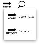
Regions can be sorted by either genome coordinates (COORD) or distances from cluster centroid (DISTANCES). To change the region sorting, click on the button and select the desired sort type. The sorting has a synergy with the histogram view: mouseover a region to indicate its location in the distance histogram.
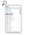
The search button brings up a search box which allows you to search for a region name and find it in the clustering. Only "Name" attributes in the GFF3 regions file are indexed for searching. As you type into the search box, all possible name matches will appear as a list, which can be selected with either:
1) Using up and down arrow keys and then press enter when the desired item is found, or
2) Scrolling through the list and clicking the desired item with the mouse.
The query string is either the currently selected item from the list of potential matches (appears in bold) or, if none is selected, then it is the typed text in the search box. A successful search results in the queried region being displayed on the far left of the Region Browser with a bold black outline. Unsuccessful queries will produce an error dialog window. Note that if two regions have the same "Name" attribute in the input regions GFF3 file, then "-1" and "-2" will be assigned to the root name to distinguish the two instances.
Useful shortcuts
Menu bar options
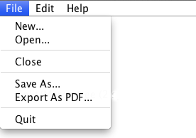
Most of these options are straightforward. However, note that Spark writes its output to a DIRECTORY (NOT a single FILE). As such, you need to select an output directory when using the "Open..." and "Save As..." options.
A more detailed description on the Export as PDF option is given at file output.
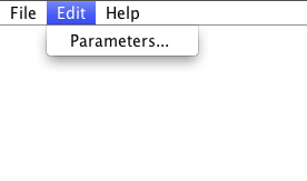
Contains the "Parameters..." option, which allow you to edit any parameter of the current analysis and save the new output. This option has been engineered to minimize the amount of computation involved. For example, changing the track colour or track order will be fast because no new data needs to be loaded. Changing the region set or the number of bins will however require reparsing the original data files and can be comparatively slow.
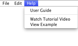
Contains links to this User Guide, a tutorial video and a precomputed Spark analysis example.
Constructing a new analysis consists of specifying three inputs:
You must specify at least one input data file ('track') for a clustering analysis. Spark provides access to data files generated by the Human Epigenome Atlas and ENCODE in addition to your own data files. Input data files can be from any organism.
Hint Currently only wig format (with file extensions '.wig', '.wig.gz', or '.wig.zip'), bigWig format (with file extensions '.bigWig' or '.bw'), and bed format (with file extensions '.bed' or '.bed.gz') are supported. BigWig format is recommended for faster loading speeds.
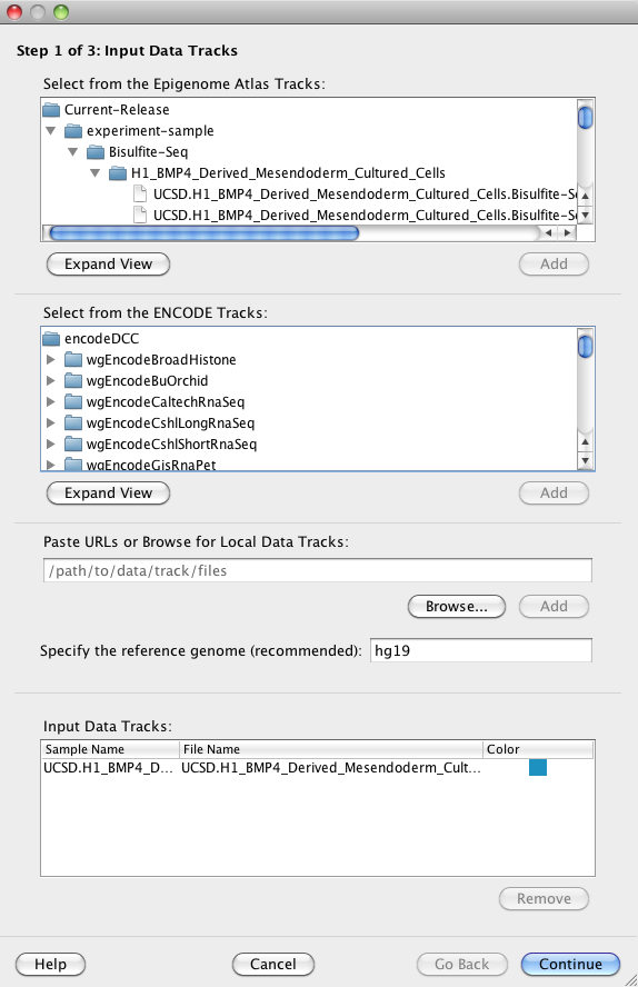
You may select one or more tracks and click on the 'Add' button to add your selections to the Input Data Tracks Table at the bottom of the panel.
Hint For the Human Epigenome Atlas tracks (top), right-clicking on a selected track will reveal a context menu with a "View metadata in GEO" option. This link will open the corresponding GEO record in your browser with all relevant information about the experiment.
This optional field allows you to specify the reference genome of your input data files (e.g. 'hg19', 'mm10', etc).
Hint Spark only uses this information when creating URL links to the UCSC Genome Browser (see section on Linking to the UCSC Genome Browser). If you have selected an Epigenome Atlas Track, then this field will default to the correct human reference genome.
This table displays information about your input data tracks. You must have added at least one track to this table to continue. The 'Sample Name' column is automatically populated with names parsed from the 'name' field in each input data file, or with the file name if this field is missing.
Hint You can double click on the Sample Names column entries to edit them. You can also modify the row order by drag-and-drop or change the display colour for each sample by using the right-click context menu in the Colour column.
You must specify a single set of region coordinates in GFF3 or BED format. Spark will cluster only data from your input data file(s) that map to these regions. These region coordinates can be for any organism, but must be compatible with the coordinates used in the input data file(s).
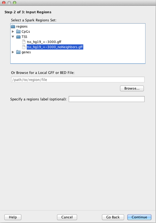
Spark provides several human region sets for your convenience. These include CpG Islands (all unique entries in the "cpgIslandExt" table from the UCSC Genome Browser), transcriptional start sites (TSS) and genes (both based on RefSeq transcripts in the "refGene" table from the UCSC Genome Browser).
In the case of TSSs, regions correspond to +/- 3 kb centered on the TSS (tss_hg19_+-3000.gff file). We also provide a filtered file in which all TSSs within 3 kb of each other are removed (tss_hg19_+-3000_noNeighbors.gff file).
Hint The Epigenome Roadmap Atlas Tracks have been preprocessed with these Spark region sets, so a clustering analysis will run faster when such a file pair is used.
Hint All regions in these sets have "Name" attributes and so are searchable by name within Spark's search box.
Alternatively, you can select one of your own region sets by clicking on the 'Browse' button. This file can be in GFF3 format and use the '.gff' extension in its file name. Briefly, each entry must contain tab delimited chromosome, source, feature, start, end, score, strand, and frame fields, followed by ";" separated attributes. For example:
chr1 ucsc TSS 26370 32369 . - . ID=NR_024540 ; Name=WASH7P
You can also use a BED file as a region input file. This file needs to be in BED format and use the '.bed' or '.bed.zip' (for zipped file) extension. Each entry must contain tab delimited chromosome, chromosome start, and chromosome end. For example:
chr1 26370 32369
Additional details, such as name, in BED files are also considered, but these are not neccesary for processing the file.
Hint The end coordinate is inclusive, e.g. a feature from 1 to 10 has a length of 10 nt (not 9 nt). The regions can be of variable length.
Hint The "Name" field is later used in the search box. In addition, the GFF3 attribute with the key "ID" is required if you want to use the interactive GO analysis feature.
This optional field allows you to label your region set. The label will be used in the window title bar in the Spark display and it can be a helpful reminder when viewing a clustering.
You must specify an output directory in which to save your results. You can modify the remaining settings or choose to use the provided defaults.
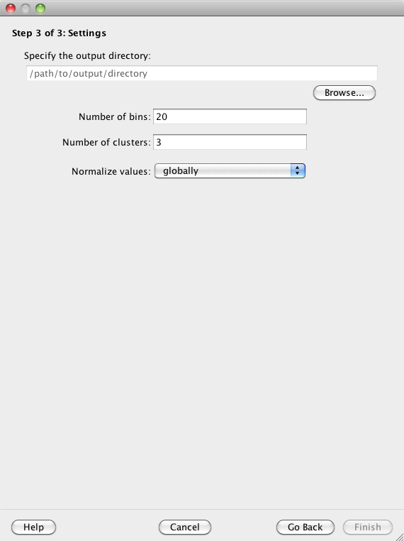
Click on the 'Browse' button to specify an output directory in which Spark will write its output files. You can later use the "File:Open..." option to select this directory and view your clustering analysis again.
Data from across the input regions are first binned prior to clustering. The "Number of bins" parameter specifies the number of (equally sized) bins to use for each region. The provided default is 20.
For example, if you use the default and your regions have variable lengths, as is the case for gene boundaries, then each gene will be divided into 20 equally sized bins for the purposes of clustering and display, but the absolute bin size in nucleotides will differ between genes.
The user must specify how many clusters Spark should initially generate. The provided default is 3. See the Split cluster control panel section to learn more about how clusters can be subsequently subdivided.
Data in each input data track are normalized separately to be in the range 0.0 to 1.0. This is important for the clustering step to ensure that equal weighting is given to the different data tracks that may have inherently different dynamic ranges.
The normalization is either done 'globally' (default) in which case the highest value across the whole genome from a given data track is assigned a 1.0, and similarly, the lowest value across the whole genome from a given data track is assigned a 0.0. In contrast, a 'regional' normalization only considers the input regions, not the whole genome. As a result, 0.0 and 1.0 indicate the minimum and maximum values, respectively, for a given data track across the input regions.
Spark employs the same normalization scheme as used by ChromaSig reported by Hon G, Ren B, and Wang W in PLoS Comput Biol. 2008 Oct;4(10):e1000201:
x'_h,i = 1/(1+e^-(x_h,i - median(x_h))/std(x_h))
for bin i and sample h. The result is that all binned values are normalized to be between 0.0 and 1.0, with a median value having a normalized value of 0.5.
Spark writes several files to the output directory that you specify. You do not need to know about their formats or functions in order to use Spark. You can simply use the graphical interface to create and open analyses. However, some of the output files may be useful to you for downstream analyses:
properties.txt
This file captures all of the parameters of your clustering analysis. If you ever wish to run Spark on the command-line, you will need to generate a properties.txt file.
clusters
There are three files inside the clusters subdirectory:
clusters.gff is identical to your input regions GFF3 file, but has been annotated to include the regions' cluster assignments (attribute "cID"). This can be a useful file if you wish to do your own downstream analyses on the clusters.
clusters.values specifies the precomputed cluster averages to display in Spark.
clusters.tree stores the split/merge tree and reloads the pathing in the next load
clusters.histogram stores the text output of the cluster histogram values
stats
Spark computes statistics (such as mean, standard deviation, etc.) for each input data file. These are calculated both globally (considering the whole input data file) and regionally (considering only the specified input regions) and are captured in the stats subdirectory as x__global.stats and x__regional.stats files, respectively.
tables
Spark stores a data table as a binary .dat file in the tables subdirectory for each input data file. Each table contains the data values from only the specified input regions. This enables Spark to avoid reparsing the input data files on subsequent reloads, thus improving performance.
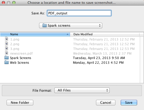
To start a PDF export, click on "File > Export as PDF.." option, or alternatively use the hotkeys Shift + P. This will bring up the first window. In this window, type in the filename and choose
the folder where you would like to save the file. Click on save to go to the next menu.
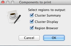
Use the checkboxes to select portion or portions of the screen to export. These portions are namely cluster summary, cluster display, and region browser. Click OK to save the file.
Running Spark on the command-line can be useful if you wish to generate many clustering analyses simultaneously (i.e. by running multiple jobs on parallel processors).
1. Download the jar file.
2. See the command-line options by running:
java -jar Spark.jar --help
You should see the following output:
Spark [version number]

Usage:
java -jar Spark.jar -p directoryPath (pre-processing mode)
java -jar Spark.jar (GUI mode)

Options:
-h [--help]              Help options
-v [--version]           Version number
-p [--preprocessing]     Specify an output directory to use
-l [--log]               Optionally specify a custom log file path and name
If no options are specified, the GUI is launched.
3. Setup your output directory:
mkdir myAnalysis
Open a properties.txt file inside this directory. This file specifies all of the parameters for your analysis. Here is an example:
#
#Wed Apr 24 14:40:26 PDT 2013
colLabels=blue,blue
dataFiles=http\://www.genboree.org/EdaccData/Current-Release/experiment-sample/Bisulfite-Seq/H1_Cell_Line/UCSD.H1.Bisulfite-Seq.combined.wig.gz,http\://www.genboree.org/EdaccData/Current-Release/experiment-sample/Histone_H3H3K4me1/Neurosphere_Cultured_Cells_Cortex_Derived/UCSF-UBC.Neurosphere_Cultured_Cells_Cortex_Derived.H3K4me1.HuFNSC02.wig.gz
statsType=global
k=3
numBins=20
includeZeros=true
regionsLabel=
randomSeed=15
sampleNames=UCSD.H1.Bisulfite-Seq.combined,UCSF-UBC.Neurosphere_Cultured_Cells_Cortex_Derived.H3K4me1.HuFNSC02
normType=exp
regionsFile=http\://www.genboree.org/EdaccData/Spark/Current-Release/regions/TSS/tss_hg19_+-3000.gff
org=hg19
Properties
dataFiles
This is a comma separated list of files that can either be local paths or URLs (or both). Currently only wig format (with file extensions '.wig', '.wig.gz', or '.wig.zip') and bigWig format (with file extensions '.bigWig' or '.bw') are supported. These are equivalent to the Input Data Tracks described above.
sampleNames
A comma separated list of sample names (in the same order as the data files above).
regionFile
A local path or URL to a single GFF3 file. This is equivalent to the Input Regions described above.
org
Reference genome (e.g. "hg19"). See a full description under Reference Genome.
regionsLabel
An optional label for your regions set. See a full description under Regions Label.
numBins
The number of bins to use per region. See a full description under Number of bins.
k
The number of clusters to generate.
normType
Specifies what type of normalization to use. Currently, Spark only provides one normalization type called "exp" which uses the same normalization scheme as ChromaSig. See the Normalization description above.
statsType
Specifies how to compute the statistics, either "global" or "regional". See the Normalization description above.
colLabels
A comma separated list of colours to use in the visualization (one per input data file). Supported options are "blue", "black", "green", "orange", "pink", and "purple".
4. Run your analysis:
java -Xms256m -Xmx1024m -jar Spark.jar -p myAnalysis
The "-Xms" and "-Xmx" specify the min and max heap size for Java. You may need to increase "-Xmx" for memory intensive jobs.
5. Open your new analysis in the graphical interface:
java -Xms256m -Xmx1024m -jar Spark.jar
Select your output directory using the "File:Open..." menu option.
We welcome you to contact us with bug reports or feedback. An error log can be found in your home directory under Spark_Cache/Spark.log. This file contains useful information regarding where the application failed.
April 2013 - Spark 1.3.0 released
Significant improvements include:
Download (via Java Web Start) Download the .jar file
August 2012 - Spark 1.2.0 released
Improvements in 1.2.0
Download (via Java Web Start) Download the .jar file
Spark was designed and implemented by Cydney Nielsen at the Michael Smith Genome Sciences Centre, BC Cancer Agency, supported by funding from CIHR and MSFHR.
Special thanks to Peter Shen from the University of Victoria for implementing the new and improved features of Spark 1.3.0, and to Hamid Younesy from Simon Fraser University for his contributions to the original codebase.
The project was developed in close collaboration with members of the NIH Roadmap Epigenomics Project and the ENCODE Project. We would like to thank Andrew Jackson and Aleksandar Milosavljevic at the Epigenome Center, Baylor College of Medicine, for integrating Spark into the Genboree Workbench.
Kindly cite your use of Spark:
Cydney B. Nielsen, Hamid Younesy, Henriette O'Geen, Xiaoqin Xu, Andrew R. Jackson, Aleksandar Milosavljevic, Ting Wang, Joseph F. Costello, Martin Hirst, Peggy J. Farnham, Steven J.M. Jones. Spark: A navigational paradigm for genomic data exploration. Genome Research. 2012 Nov;22(11):2262-9.
For all help questions, bug reports, feature requests, and other suggestions, we encourage you to use our spark_users group.
If you need to contact the Spark team privately on other topics, you can email us directly.